Chapter 7 Autoregressive models
7.1 Principle of ARMAX models
Most of the data recorded by monitoring buildings are time series: sequences taken at successive points and indexed in time. The previous chapter dealt with data that were aggregated with low enough frequency that successive values of the outcome variable could be considered independent from each other, and only dependent on explanatory variables. This aggregation however comes with a significant loss of information, since all dynamic effects are smoothed out. Dynamic models, including time-series models, allow the dependent variable to also be influenced by its own past values.
Autoregressive models are based on the idea that the current value of the series, \(y_t\), can be explained as a function of \(p\) past values, \(y_{t-1}\), \(y_{t-2}\), …, \(y_{t-p}\) where \(p\) determines the number of steps into the past needed to forecast the current value. The simplest time-series models are linear AutoRegressive (AR) models. The AR(p) model is of the form: \[\begin{equation} y_t = \alpha + \beta_1 y_{t-1} + \beta_2 y_{t_2} + ... + \beta_p y_{t_p} + \epsilon_t \tag{7.1} \end{equation}\] where \(\epsilon_t \sim N(0, \sigma^2)\) is independent identically distributed (iid) noise with mean \(0\) and variance \(\sigma^2\). This notation is equivalent to writing: \[\begin{equation} y_t \sim N(\alpha + \beta_1 y_{t-1} + \beta_2 y_{t_2} + ... , \sigma^2) \tag{7.2} \end{equation}\] but the time-series literature usually separates the noise into a dedicated variable \(w_t\) in order to formulate assumptions for it.
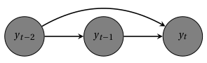
Figure 7.1: AR(2) model: an observation is conditioned on its two previous instances
AR models can be extended into many forms, including the AutoRegressive (AR) Moving Average (MA) model with eXogeneous (X) variables, or ARMAX. In addition to being related to its own \(p\) previous values AR(p), the output can be predicted by additional inputs (X) and the white noise \(\epsilon_t\) can be replaced by a moving average of order \(q\) MA(q): \[\begin{equation} E(y_t|\theta, X) = \sum_{i=1}^p \beta_i y_{t-i} + \sum_{j=0}^q \gamma_j \epsilon_{t-j} + \sum_{k=1}^K \left[ \sum_{i=0}^p \theta_{k,i} x_{t-i,k} \right] \tag{7.3} \end{equation}\] On the right side of this equation, the second term, MA(q), is a linear combination of the successive values of the prevous errors. The third term includes the influence of the current value and up to \(p\) previous values of \(K\) explanatory variables. A more general notation could assume a different order \(p\) for each separate input.
ARX and ARMAX models have among others been applied to modelling the heat dynamics of buildings and building components by the collaborative work of the IEA EBC Annex 58 (Madsen et al. (2015)). Issues when applying AR(MA)X-models are not only the selection and validation of the model, but also the extraction of physical information from the model parameters, as each individual parameter lacks a direct physical meaning. An important step in ARX-modelling is to select suitable orders of the input and output polynomials. This can be done by stepwise increasing the model order until most significant autocorrelation and cross correlation are removed.
We refer to the books of Madsen (Madsen (2007)) or Shumway et al. (Shumway and Stoffer (2000)), for a more extensive description of all types of AR models. Further structures include Integrated models for non-stationary data (ARIMA), Seasonal components for longer-term cyclic data (SARMA, SARIMAX), and the autoregressive conditionally heteroscedastic (ARCH) model for non-constant conditional noise variance.
7.2 Tutorial (Rstan)
Auto-regressive models are covered in the Stan user’s guide. In this chapter and the next few ones, we demonstrate their use for the prediction of energy consumption.
7.2.1 Data: the ASHRAE machine learning competition
In 2019, the ASHRAE great energy predictor competition was featured on Kaggle. Participants developed models of metered building energy usage: chilled water, electric, hot water, and steam meters. The purpose of the competition was to find good modelling options for M&V and encourage energy-saving investments.
The data comes from over 1,449 buildings over a three-year timeframe, located in 16 different North-American sites. The dataset also includes basic weather data of all sites and some metadata for each building. Only a few buildings have all four meter types. In this chapter, one of these buildings was picked, labeled Building 1298.
All examples of the Times-series modelling part of this book (autoregressive models and hidden Markov models) will be illustrated with the Building 1298 data. The complete dataset of the competition is available on Kaggle, but the data for this particular building has been extracted and is shared in the book’s repository.
The following figure shows the readings of all 4 meters of this building during the whole training dataset. You can zoom in or hide some of the lines with the bokeh toolbar on the right.
We start by importing libraries and the data file, and by looking at its content with the head() function.
library(rstan)
library(tidyverse)
library(lubridate)

df <- read.csv("data/building_1298.csv")

head(df)
## datetime m0 m1 m2 m3 air_temperature
## 1 2016-01-01 00:00:00 416.169 1994.63 2334.99 0.0000 5.6
## 2 2016-01-01 01:00:00 408.616 2101.56 2755.43 79.5127 5.6
## 3 2016-01-01 02:00:00 412.072 1885.37 2564.32 0.0000 5.6
## 4 2016-01-01 03:00:00 393.053 1909.73 2804.94 0.0000 5.6
## 5 2016-01-01 04:00:00 404.519 1882.42 2621.65 132.9570 5.0
## 6 2016-01-01 05:00:00 406.975 1700.60 3047.30 74.5527 4.4
## cloud_coverage dew_temperature precip_depth_1_hr sea_level_pressure
## 1 0 -0.6 0 1019.3
## 2 0 -0.6 0 1019.3
## 3 4 -0.6 0 1019.4
## 4 NA -1.1 0 1019.4
## 5 NA -2.2 0 1019.2
## 6 NA -2.2 0 1018.9
## wind_direction wind_speed
## 1 300 2.6
## 2 300 2.6
## 3 300 2.6
## 4 NA 1.5
## 5 290 3.1
## 6 300 4.1In this pre-processed data file, the meter readings are called m0 to m3 and there is a number of weather variables to choose explanatory variables from. The time resolution is hourly, which justifies the use of time series models.
The following block performs some additional data processing and selection. First, we add some separate variables to the dataframe: the date, hour, day of week of each line. Also, the fill() function replaces NaN values found in some columns. Then, two subsets of the dataframe are chosen as separate training and test dataframes df.train and df.test. In the original Kaggle competition, the whole year of readings shown above is just the training period. We chose a shorter training and testing period within this original training data so that we can later show how the model performs in prediction.
df <- df %>%
  mutate(Date = as_date(datetime),
         hour = hour(datetime),
         wday = wday(Date),
         week.end = wday==1 | wday==7) %>%
  fill(air_temperature, wind_speed)

trainingStart <- as.Date("2016-05-01", "%Y-%m-%d")
trainingEnd <- as.Date("2016-05-31", "%Y-%m-%d")
testEnd <- as.Date("2016-06-07", "%Y-%m-%d")
df.train <- df %>% filter(datetime > trainingStart, datetime < trainingEnd)
df.test <- df %>% filter(datetime > trainingStart, datetime < testEnd)
7.2.2 A simple ARX model
The complete equation for an AR(p)MA(q)X model is shown by Eq. (7.3). Below, we will use a slightly simpler version of this model: the moving average term is left out as it is difficult to physically justify its relationship with meter readings. The following is therefore an ARX model defined with Stan, where \(P\) is the autoregressive order, and there are \(K\) explanatory variables. At every time step, we suppose that the current and the \(P\) previous values of the explanatory variables can be used: this means that the parameter \(\theta\) is a \((P+1) \times K\) matrix.
model = "
data {
  int<lower=0> N_train;     // data points (training)
  int<lower=0> N;           // data points (all)
  int<lower=0> K;       // number of predictors
  int P;                // AR order

  matrix[N, K] x;       // predictor matrix (training and test)
  vector[N_train] y;    // output data
}

parameters {
  real alpha;                 // mean coeff
  row_vector[P] beta;         // AR parameters
  row_vector[P+1] theta[K];   // coefficients of explanatory variables
  real<lower=0> sigma;        // error term
}

model {
  for (n in P+1:N_train) {
    real ex = 0;
    for (j in 1:K)
        ex += theta[j] * x[n-P:n, j];
    y[n] ~ normal(alpha + beta * y[n-P:n-1] + ex, sigma);
    }
}

generated quantities {
  vector[N] y_new;

  for (n in 1:P)
    y_new[n] = y[n];

  for (n in P+1:N_train) {
    real ex = 0;
    for (j in 1:K)
        ex += theta[j] * x[n-P:n, j];
    y_new[n] = normal_rng(alpha + beta * y[n-P:n-1] + ex, sigma);
  }

  for (n in N_train+1:N) {
    real ex = 0;
    for (j in 1:K)
        ex += theta[j] * x[n-P:n, j];
    y_new[n] = normal_rng(alpha + beta * y_new[n-P:n-1] + ex, sigma);
  }
}
"
The generated quantities block at the end of this model computes the predicted output of the model every time a sample has been generated. This is an interesting feature of Stan to easily calculate posterior probabilities of variables other than the model’s parameters. The y_new variable will be used to assess the prediction performance of the fitted model.
The next steps are similar to the other Stan examples given in this book:
- A
model.datalist is created to map the data from the dataframes to the Stan model; - Model fitting;
- Printing posterior distributions of parameters and saving results in a dataframe.
In this example, the outdoor air temperature was picked as the only explanatory variable, and the autoregressive order is only 1.
model.data <- list(
  N_train = nrow(df.train),  # number of training data points
  N = nrow(df.test),         # total number of data points
  K = 1,                     # number of predictors
  P = 1,                     # AR order
  y = df.train$m0 ,          # dependent variable (training data)
  x = df.test %>% select(air_temperature) # explanatory variables (all data)
)

fit <- stan(
  model_code = model,  # Stan program
  data = model.data,        # named list of data
  chains = 4,               # number of Markov chains
  warmup = 1000,            # number of warmup iterations per chain
  iter = 2000,              # total number of iterations per chain
  cores = 2,                # number of cores (could use one per chain)
  refresh = 1,              # progress not shown
)

print(fit, pars=c("alpha", "beta", "theta", "sigma"))
## Inference for Stan model: 4800e29de0bb5622caa49441804892bc.
## 4 chains, each with iter=2000; warmup=1000; thin=1;
## post-warmup draws per chain=1000, total post-warmup draws=4000.
##
## mean se_mean sd 2.5% 25% 50% 75% 97.5% n_eff Rhat
## alpha 195.40 0.38 14.04 167.40 186.03 195.26 205.21 222.13 1373 1
## beta[1] 0.57 0.00 0.03 0.51 0.55 0.57 0.59 0.63 1358 1
## theta[1,1] -5.97 0.03 1.26 -8.38 -6.84 -6.00 -5.12 -3.50 1567 1
## theta[1,2] 5.99 0.03 1.26 3.48 5.17 6.02 6.86 8.42 1575 1
## sigma 37.53 0.02 0.99 35.67 36.84 37.49 38.18 39.56 2344 1
##
## Samples were drawn using NUTS(diag_e) at Wed Jul 06 14:39:39 2022.
## For each parameter, n_eff is a crude measure of effective sample size,
## and Rhat is the potential scale reduction factor on split chains (at
## convergence, Rhat=1).This model is simple enough to reach convergence without any priors, but they would quickly become necessary if the number of unknown parameters were to increase.
Finally, we can look how well the fitted model predicts the dependent variable, since some test data was extracted from the original dataframe. The prediction y_new was directly calculated by Stan in the generated quantities block: each sample of the posterior comes with a predicted output. We can therefore display the quantiles of the posterior predictive distribution as follows:
# Saving results in a dataframe
la <- rstan::extract(fit, permuted = TRUE)

# Quantiles from the posterior predictive distribution
y.quantiles <- apply(la$y_new, 2, quantile, probs=c(0.025, 0.5, 0.975))
df.test <- df.test %>%
  mutate(pred_low = y.quantiles[1, ],
         pred_med = y.quantiles[2, ],
         pred_up = y.quantiles[3, ])

# Plot
plotStart <- as.Date("2016-05-23", "%Y-%m-%d")
plotEnd <- testEnd
ggplot(data = df.test %>% filter(datetime > plotStart, datetime < plotEnd)) +
  geom_line(mapping = aes(x=ymd_hms(datetime), y=m0)) +
  geom_line(mapping = aes(x=ymd_hms(datetime), y=pred_med), color="red") +
  geom_ribbon(mapping = aes(x=ymd_hms(datetime), ymin=pred_low, ymax=pred_up), fill='red', alpha=0.1)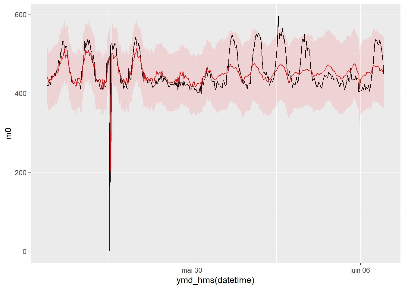
This plot shows the predicted output during the last week of the training period (until the end of May) and during the test period (beginning of June). We can see that as soon as baseline data stops being available, the model reproduces some trend in the data but doesn’t perform very well.