Chapter 1 Background on data analysis
1.1 The energy savings potential of buildings
The energy consumption of buildings accounts for 40% of the global primary energy use and up to 33% of carbon emissions in some countries, mainly from the operation of heating, ventilation and air conditioning (HVAC) systems. The gap in energy performance between older, poorly insulated constructions, and newer net-zero energy or passive buildings with efficient energy control strategies, shows the magnitude of the improvement that could be brought to the energy efficiency of the building stock. It is commonly known that the share of new buildings in the overall construction sector is very low. Most buildings are several decades old and often have poor energy performance, especially compared to recent standards for new constructions. The largest potential for energy savings in the building sector therefore lies in the renovation of the existing building stock, or its proper energy management.
Data science offers promising prospects for improving the energy efficiency of buildings. Thanks to the availability of smart meters and sensor networks, along with increasingly accessible algorithms for data processing and analysis, statistical models may be trained to predict the energy use of HVAC systems or the indoor conditions. These trained models and their predictions then lead to various inferences: assessing the real impact of energy conservation measures; identifying HVAC faults or physical properties of the envelope in order to provide incentive for retrofitting; minimizing energy consumption through model predictive control; detecting and diagnosing faults; etc.
The availability of measurements and computational power have given data mining methods an increasing popularity. The field of data analysis applied to building energy performance assessment however faces two main challenges to this day. Ironically, the first challenge is the abundance of data. Smart meters and building management systems deliver large amounts of information which can hide the few readings which are the most relevant to energy conservation. Automated monitoring and fault detection algorithms only do what they are told, and will hardly replace human intervention when it comes to understanding readings. The second challenge is the difficulty of data science. Without a principled methodology, it is very easy to draw erroneous conclusions, by incorrectly assuming that a model is properly trained. By lack of a background in statistics, building energy practitioners often lack the tools to ensure their inferences are correct.
1.2 From data to energy savings
1.2.1 Formalisation of the system
Before proposing a few examples on how data acquisition may support energy conservation measures, let us first formalise the framework, in which the following parts of this book will describe building energy performance.
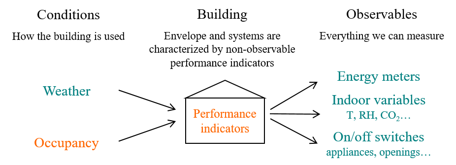
Figure 1.1: Formalisation of the system into observable variables and non-measurable influences
The first level of this formalisation are the two conditions imposed on the building: weather and occupancy. What these two terms have in common is the fact that the building’s designer does not get to choose or influence them: every analysis that we will conduct will be conditional on these imposed conditions.
The weather imposes the outdoor boundary conditions of the building envelope. It can be described as a set of measurable quantities (outdoor air temperature, humidity, direct and diffuse solar irradiance, wind speed and direction…), some of which are predictable to some extent. The occupancy is more difficult to extensively describe with a finite set of variables. This term is used here to encompass all actions and choices of the occupants regarding their own comfort and how they “operate” the building: leaving and entering the building, setting indoor temperature set points, opening and closing windows, operating appliances that consume energy… These actions cannot be simply measured and summarised into a few descriptive variables, as can be the weather.
The second level of the formalisation is the building itself. Building energy simulation usually separates the description of the HVAC systems and the envelope. Both can be characterised in terms of energy performance by a finite set of intrinsic performance indicators: heat transfer coefficient of the envelope, boiler efficiency, window transmissivity, pipe network heat loss… These quantities cannot be directly observed, and define the intrinsic energy performance of the building: their values should not depend on the current state of the two previously mentioned conditions.
The third level of the formalisation includes all extensive and intensive variables that can be measured by any kind of meter or sensor, inside or near the building. These variables are the consequences of the two conditions (weather and occupancy) coupled with the building’s intrinsic performance. They include readings from energy meters, variables which describe the indoor air (temperature, relative humidity, CO\(_2\) concentration…) and various signals that describe the state of operation of HVAC systems or envelope components. The indoor air temperature, for instance, is influenced by the weather (outdoor air temperature, solar irradiance), the occupants (who chose the set point) and the intrinsic building energy performance (heat transfer coefficient and inertia of the envelope, efficiency of the temperature control loop). These variables, along with weather variables, constitute the data from which we will perform inferences and predictions.
1.2.2 Some uses of data
We now use this formalisation to demonstrate a few examples of how recorded data may be used to motivate energy conservation measures or verify their efficiency. Fig. 1.2 uses the same color code as Fig. 1.1: blue denotes observable variables, orange denotes non-measurable information.
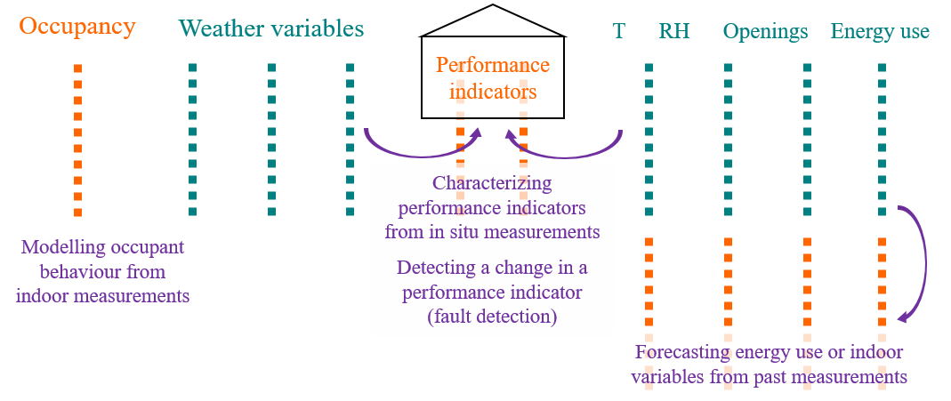
Figure 1.2: How data can be used for various inferences and predictions
- Forecasting energy use
The ability to predict the energy use of buildings is a useful tool for energy management, from the scale of a single dwelling to the scale of energy distribution in a smart grid. On a side note, we can mention a difference between the terms of prediction and forecasting. In modelling studies, prediction is a general term that means computing the outcome of any simulation model, while forecasting specifically denotes estimating the future values of a time series, on a time horizon where observations are not available.
Two factors may facilitate the ability to forecast a time series. The first of these advantageous characteristics is a repetitive trend in an energy consumption profile (see Fig. 1.3). Large office buildings, collective housing and retail facilities tend to display a predictable daily profile for energy uses that have a low dependency on environmental factors, such as lighting and electrical appliances. Some energy uses mostly depend on user behaviour, whose stochastic behaviour tend to be smoothed out at larger scales of observation.
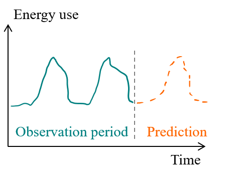
Figure 1.3: Repetitive consumption profiles are easy to forecast by extrapolating daily and seasonal fluctuations
Another factor that facilitates the prediction of energy use is a high dependency on an environmental factor that is itself easy to get forecasts of. In a building with a controlled set-point indoor temperature, a strong correlation may be observed between the outdoor temperature and the heating power in winter (see Fig. 1.4). The outdoor temperature is then considered a significant explanatory variable: its forecasts will allow forecasting the heating power with a satisfactory confidence.
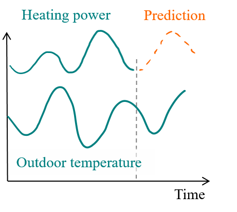
Figure 1.4: A correlation between outdoor temperature and heating power can be used to predict future demand
These two examples illustrate two categories of leverages in time series analysis and forecasting. When forecasting a particular series, we can either make use of its own characteristics (periodicity, seasonality, autocorrelation…), or identify dependencies with other measurable data.
- Measurement and verification (M&V)
The ability to predict energy demand can also be valued in the context of Measurement and Verification (M&V). M&V is the process of assessing savings caused by an Energy Conservation Measure (ECM). Savings are determined by comparing measured consumption or demand before and after implementation of a program, making suitable adjustments for changes in conditions. The International Performance Measurement and Verification Protocol (IPMVP) formalizes this process, and presents several options to conduct it.
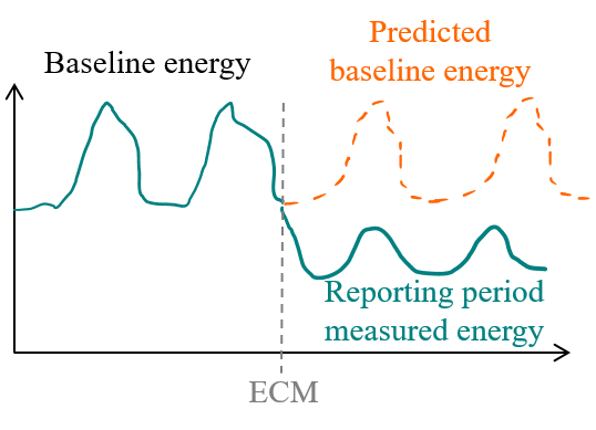
Figure 1.5: The IPMVP provides guidelines on how to perform M&V
An example of adjustment is, when estimating the energy savings delivered by an ECM, to substract its new energy consumption from the consumption that would have occurred if the building had stayed in the same situation in the weather conditions of the reporting period (adjusted baseline consumption). This requires a prediction model that can extrapolate the initial behaviour of the building by accounting for variable weather conditions. Other possible adjustments include changes in occupancy schedules. This is necessary to assess whether measured energy savings are caused by the ECM itself, or by changes in these influences.
The IPMVP presents several options, depending on whether the operation concerns an entire facility or a portion, and defines the notion of measurement boundary as the set of measurements that are relevant to determine savings. In order to verify the savings from a single equipment, and a measurement boundary can be drawn around it, the approach used is retrofit-isolation: IPMVP options A and B. If the purpose of reporting is to verify total facility energy performance, the approach is the whole-facility option C. All options must account for the presence of interactive effects: energy impacts created by the ECM that cannot be measured within the measurement boundary. Any option that requires adjustment on measured independent variables implies the use of a prediction model, even a simple one. In the IPMVP option D, savings are determined through simulation of the energy consumption rather than direct measurements. The simulation model is calibrated so that it predicts the energy and load that matches the actual metered data. Under the correct assumptions, and with the right methodology (which we propose in this book!), calibrated simulation is potentially a very powerful M&V methodology, as it may disaggregate energy uses and estimate interactive effects outside of the measurement boundary.
M&V is a crucial tool in the establishment of Energy Performance Contracts (EPC), which can be established on the basis of designed performance (building energy simulation), with an eventual uncertainty analysis and/or sensitivity analysis, or on the basis of measured energy consumption.
- Intrinsic performance assessment
The third hereby presented application of data analysis is the estimation of quantitative indicators of the intrinsic energy performance of a building. This is different from the M&V process as it does not necessarily imply the comparison between before/after situations. One typical example is the Heat Loss Coefficient (HLC), or the Heat Transfer Coefficient, which characterize heat transmission through the envelope, eventually including air infiltration. The co-heating test is one of the well-known methods for HLC assessment: it measures the heating power required to maintain a steady indoor temperature, and obtains HLC by averaging these measurements over a sufficiently long period.
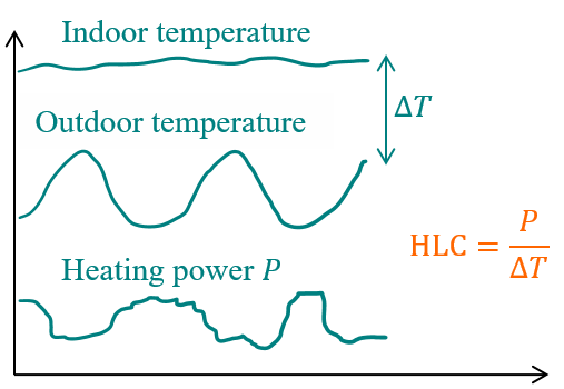
Figure 1.6: The co-heating test records the heating power, indoor and outdoor temperature, in order to estimate the heat loss coefficient of the envelope
What is referred here as intrinsic performance assessment may also be called characterization, or parameter estimation, since it primarily works by estimating the values of static parameters of a simulation model. Such parameters may include the HLC, but also the efficiency of a system, an air infiltration rate… Hence, it can be part of an energy audit to help characterize the state of a building and its eventual flaws before the design of an ECM.
- Fault detection and diagnostics
One of the characteristics of “smart buildings” is the ability to monitor energy usage with the aim of identifying abnormal consumption behaviour and notifying the building manager to implement appropriate procedures (Araya et al. (2017)). Fault detection and diagnostics (FDD) is the process of using building operational data to detect the occurence of faults and identify their root causes (Granderson et al. (2020)). This process can be done manually, or by an algorithm delevoped to perform it automatically.
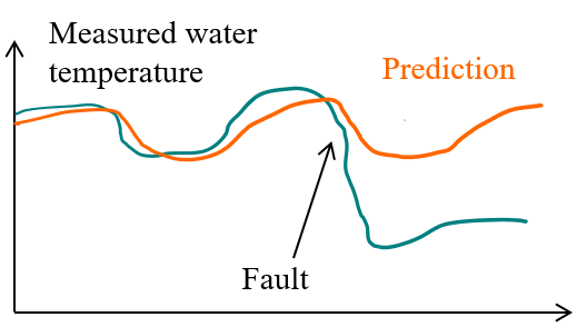
Figure 1.7: Fault detection is a double challenge: (1) automatically detecting a difference between measurements and normal behaviour; (2) identifying its possible cause.
Many supervised statistical learning methods for building energy load forecasting and anomaly detection have been developed in the last years. FDD is a challenging topic because it needs to reconcile two targets: efficient pattern detection among possibly large amounts of data, and physical interpretability of detected anomalies based on a detailed description of the building and its components.
1.2.3 Model calibration as the key to data analysis
All the applications described above can be summarized by the same description: data are recorded and interpreted to draw conclusions about quantities that are either not directly observable (such as estimating a heat loss coefficient), or not yet observed (such as forecasting energy use). In all cases, the missing link between the data and the conclusion is a numerical model.
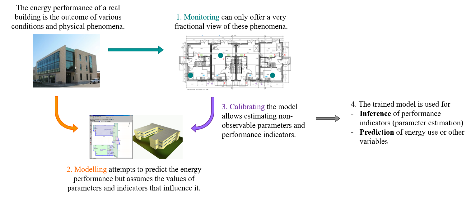
Figure 1.8: The overall process of collecting and analyzing data
As was described by the formalisation proposed above, the energy consumption of HVAC systems and other appliances, along with other measurable indoor variables, are the consequences of two sets of conditions (weather and occupancy) and of the intrinsic energy performance of the envelope and systems. Disaggregating each of these influences, and accessing intrinsic energy performance indicators, is a major challenge. For instance, measurement and verification protocols attempt to demonstrate whether energy savings may be attributed to an energy conservation measure, or is partially caused by a change in weather or occupancy behaviour.
After identifying the phenomena that we wish to predict, or the performance indicators that we wish to estimate, monitoring equipment is implemented for data acquisition. Measurements are an insight of the real behaviour of a building, and are the basis for training the models that will reproduce it. The required types of monitoring depend on the characterisation target and on the specific energy uses of the building under study. In all cases, measurements can only provide a very fractional view of all phenomena that drive the energy performance. Heating and cooling energy consumption, for instance, is the outcome of several concurring heat transfer phenomena: transmission through the envelope and between thermal zones; convection through ventilation and air infiltration; temperature stratification inside each room; long-wave radiative heat exchange between walls… Heating and cooling are also not the only energy consumptions that an operator may wish to be able to predict. Unless separate energy meters are implemented on each system and appliance, measurements of energy consumption are often aggregated values from which separate uses are difficult to isolate. Other important characteristics of the monitoring equipment are: the type and accuracy of sensors used for a given measurement, the acquisition time step, the spatial granularity of observation.
Raw data only describes a fraction of the overall system, and does not allow disaggregating intrinsic energy performance indicators from influences of the weather and of the occupants. The solution to this problem is to define a numerical model as the missing link between the complexity of the real building and the conciseness of the data. The model is a numerical description of the building, where the non-observable performance indicators are given a specified value. The conditions imposed by the weather and the occupants are quantified in the equations of the model, which in turn provides values for energy consumption or indoor variables as output. Model specification is all but trivial, especially because of the variety of model types offered by building energy simulation. Selecting an appropriate model structure is essential to the learning procedure. The complexity of the model is a compromise between realism and parcimony: it should at least describe all the most significant processes occuring in the system, and should not allow any redundancy in the input-output relationship. Among several models, equally capable of reproducing a dataset, the best choice is usually the most simple one (Hastie, Tibshirani, and Friedman (2009)).
The model is first defined after our knowledge of the state of the building. The next step is its calibration using the measured data. Calibrating a model means finding the settings or set of parameters with which its output best matches a series of observations, called a training dataset. This data usually originates from measurements (in either experimental test cells or real buildings), but may also have been produced by a complex reference model that we wish to approximate by a simplified one. There are two main outcomes of model training, which were already shown by two categories of data analysis applications:
- The first outcome are inferences about the processes that generated the data. If the model structure was appropriately chosen for this purpose, its parameters are related to the intrinsic energy performance indicators of the building.
- The second outcome is the ability acquired by the model to reproduce measurements, and therefore forecast the future values of some of the observed variables.
Model calibration is therefore the key to all applications of data analysis that we mentioned earlier. It is however a more complicated problem than it seems and requires careful choices at every step of the entire procedure.
1.2.4 The difficulty of inverse problems
Inverse techniques are a suite of methods which promise to provide better experiments and improved understanding of physical processes. Inverse problem theory can be summed up as the science of training models using measurements. The target of such a training is either to learn physical properties of a system by indirect measurements, or setting up a predictive model that can reproduce past observations. In the last couple of decades, building physics researchers have benefited from elements of statistical learning and time series analysis to improve their ability to construct knowledge from data. What is referred to here as inverse problems are actually a very broad field that encompasses any study where data is gathered and mined for information. Inverse heat transfer theory (Beck, Blackwell, and Clair Jr (1985)) was developed as a way to quantify heat exchange and thermal properties, and has translated well into building physics.
Many engineers and researchers however lack the tools for a critical analysis of their results. This caution is particularly important as the dimensionality of the problem (i.e. the number of unknown parameters) increases. When data are available and a model is written to get a better understanding of it, it is very tempting to simply run an optimisation algorithm and assume that the calibrated model has become a sensible representation of reality. If the parameter estimation problem has a relatively low complexity (i.e. few parameters and sufficient measurements), it can be solved without difficulty. In these cases, authors often do not carry a thorough analysis of results, their reliability and ranges of uncertainty. However, it is highly interesting to attempt extracting the most possible information from given data, or to lower the experimental cost required by a given estimation target. System identification then becomes a more demanding task, which cannot be done without proof of reliability of its results. One should not overlook the mathematical challenges of inverse problems which, when added to measurement uncertainty and modelling approximations, can easily result in erroneous inferences.
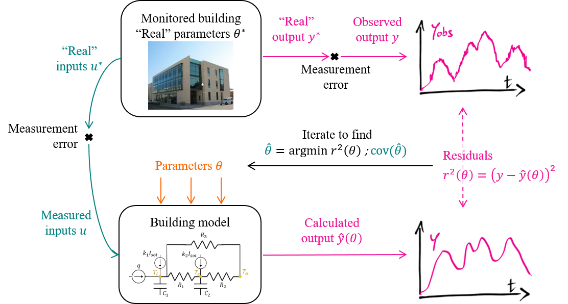
Figure 1.9: Inverse problems in a nutshell
Following the formalisation of building energy monitoring shown above, we propose a formalisation of a typical inverse problem for building physics (Rouchier (2018)), without considering any statistical aspects for now.
The general principle of solving a system identification problem is to describe an observed phenomenon by a model allowing its simulation. Measurements \(\mathbf{z}=(\mathbf{u},\mathbf{y})\) are carried in an experimental setup: a building is probed for the quantities from which we wish to estimate its energy performance (indoor temperature, meter readings, climate, etc.) A model is defined as a mapping between some of the measurements set as input \(\mathbf{u}\) (boundary conditions, weather data) and some as output \(\mathbf{y}\). A numerical model is a mathematical formulation of the outputs \(\hat y(u, \theta)\), parameterised by a finite set of variables \(\theta\). The most intuitive way to calibrate a model is to minimize an indicator such as the sum of squared residuals with an optimisation algorithm, in order to find the value of \(\theta\) that makes the model most closely match the data.
Ideally, the model is unbiased: it accurately describes the behaviour of the system, so that there exists a true value \(\theta^*\) of the parameter vector for which the output \(\hat y\) reproduces the undisturbed value of observed variables. \[\begin{equation} \mathbf{y}_k = \mathbf{\hat y}_k(u, \theta^*) + \varepsilon_k \tag{1.1} \end{equation}\] where \(\varepsilon\) denotes measurement error, i.e. the difference between the real process \(y^*\) and its observed value \(y\). The most convenient assumption is that of additive noise, i.e. \(\varepsilon_k\) is a sequence of independent and identically distributed random variables.
In practice, \(\theta^*\) will never be reached exactly, but rather approached by an estimator \(\hat \theta\), because the entire process of estimating it from measurements is disturbed by an array of approximations (Maillet (2010))
- Experimental errors. The numerical data \((u,y)\) available for model calibration differs from the hypothetical outcome of the ideal, undisturbed physical system \((u^*,y^*)\). Sensors may be intrusive, produce noisy measurements, may be poorly calibrated, have a finite precision and resolution…
- Numerical errors. The hypothesis of an unbiased model (Eq. (1.1)) states that there exists a parameter value \(\theta^*\) for which the model output is separated from the observations \(y\) only by a zero mean, Gaussian distributed measurement noise. It means that the model perfectly reproduces the physical reality, and the only perceptible error is due to the imperfection of sensors. This is exceedingly optimistic, especially in building energy simulation.
Measurement and modelling approximations are problematic because inverse problems are typically ill-posed (Beck, Blackwell, and Clair Jr (1985)): their solution is highly sensitive to noise in the measured data and approximation errors. A global optimum of the inverse problem may then be found with unrealistic physical values for \(\theta\) as a consequence of seemingly moderate errors made when setting up the problem.
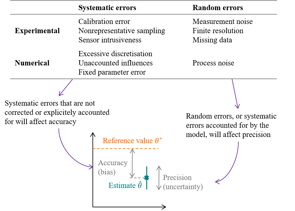
Figure 1.10: Errors and uncertainties on parameter estimation, caused by measurement and modelling errors
We divided source of errors into experimental and numerical errors. The Guide to the expression of Uncertainty in Measurement (GUM)(JCGM (2008)) then separates errors into a random component and a systematic component: systematic errors are errors which retain a non-zero mean if the measurement was repeated an infinite number of times under repeatability conditions. Systematic and random errors, whether they concern the measurement or the modelling procedures, will affect the estimation of a parameter \(\theta\) in terms of accuracy and precision. The figure above illustrates accuracy and precision in the case of estimating a parameter value \(\theta\), but the exact same terminology can be used if the purpose of the trained model is to predict the future values of a variable \(y\).
- The GUM defines uncertainty (of measurement) as the dispersion of the values that could reasonably be attributed to a measured quantity. Similarly, parameter estimates or model predictions come with an uncertainty, which quantifies their possible range of values caused by the random errors in the measurement and modelling processes. Precision is an indicator of low uncertainty, and can be conveyed by confidence intervals.
- On the other hand, accuracy is a measure of bias. It is the difference between the “true” value of the target variable and the mean of our estimation.
Biased estimates and predictions are the outcome of errors that have not been explicitely taken into account in the inverse problem. We tend to prefer low bias and high uncertainty, than high bias and low uncertainty: indeed, a high uncertainty suggests that the data were not sufficient to provide confident inferences, which incites caution when communicating the results. On the contrary, the bias cannot be simply estimated and is not visible. The worst case scenario is obtaining a bias higher than the uncertainty, which means that the true reference value is not even contained in our confidence interval. By including possible systematic errors in the model formulation, we wish to “turn bias into uncertainty”.
In order to ensure, as much as possible, that the parameters and predictions returned by the model calibration procedure are unbiased and physically interpretable, a complete workflow will be described in the next chapter of this book. This workflow sums up the important steps that should be followed before and after applying the training algorithm itself, and the various tests to be performed to prevent biased conclusions. Statistical modelling will give us the tools to perform such a careful analysis of data.
1.3 Categories of data-driven modelling approaches
1.3.1 Either physical interpretability or prediction accuracy
The main subject of this book is to propose a workflow for the analysis of building energy data, that attempts to make the most out of the available data while avoiding the inherent pitfalls of inverse problems. This workflow is described and applied in the parts of the book that follow. Before presenting it, it is however perhaps necessary to clarify some aspects of vocabulary.
The previous sections have used expressions that seemed interchangeable, or at least overlapping in their definitions: model calibration; data-driven modelling; statistical learning and inference; inverse problems… These terms can describe the same process, or a part of it: collecting data and interpreting them with a numerical or a statistical model, in order to draw conclusions that will support energy conservation measures. There is so much literature on data-driven approaches for forecasting building energy consumption and demand, that several reviews are made every year, and a review of these reviews could be done. One noticeable trend is to classify models into white-box, grey-box and black-box (Deb and Schlueter (2021)), according to their physical interpretability.
A classification of data analysis methods and terms is proposed here: models categories from white-box to black-box are shown on a scale of two criteria: physical interpretability and forecasting accuracy. They are then roughly separated into three types of approaches: model calibration (mostly for white-box models), machine learning (black-box) and statistical learning with (grey-box) probabilistic models).
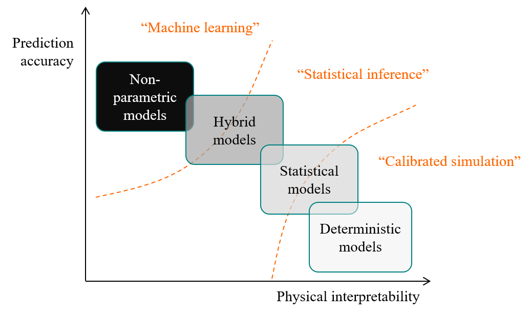
Figure 1.11: Data analysis methods can be split into three categories.
The first criterion by which methods can be classified is their requirements. These applications shown above essentially have at least one of the following two requirements:
- Applications that require the ability to accurately forecast the energy use, or any other variable: energy management, optimised predictive control. These applications do not need the trained predictive model to have physically interpretable parameters, or even parameters at all.
- Applications that involve learning the value of one or more interpretable physical values that describe physical properties of a building. These applications, such as the co-heating test, may be denote performance assessment or characterisation.
Some applications require both prediction accuracy and physical interpretability to some extent: measurement and verification, commissioning, fault detection…
The requirement of data analysis will determine the type of model that will be trained to replicate the data. The type of model is then closely related to the way that inferences will be drawn from it. We can loosely classify data analysis workflows into the three following categories:
1.3.2 Calibrated simulation (white-box)
Model calibration usually denotes fitting numerical models which are based on a more or less detailed physical description of the building, complete with a description of HVAC systems and controls, usually without a statistical representation of variables. The advantage of these models is their interpretability: each parameter has a direct meaning, which can be related to thermophysical properties of the envelope or systems. The IPMVP Option D evaluates energy savings by directly adding or removing energy conservation measures in a calibrated numerical model, and therefore requires such a detailed description of the building.
Detailed building energy models can be trained to replicate data by manual adjustement of parameters, or by more automated methods (Reddy (2006)). The ASHRAE Guideline 14 specifies what is an acceptable level of accuracy or uncertainty for a calibrated simulation with very permissive criteria: “typically, models are declared to be calibrated if they produce Mean Bias Errors (MBE) within 10% and CV(RMSE) within 30% when using hourly data, or 5% MBE and 15% CV(RMSE) with monthly data.”
Calibrating detailed models however comes with conditions and limitations. A sufficiently detailed model, with enough degrees of freedom, will have no difficulty satisfying the above criteria, but may do so without necessarily assigning their true physical value to each parameter. This inverse problem may have identifiability issues, i.e. the existence of infinitely many combinations of different parameters which result in the same model output. A preliminary sensitivity analysis may be conducted in order to only select the most significant parameters as free for calibration, while fixing the rest. Still, deterministic models greatly underestimate the bias and uncertainty of their own predictions, and calibrated simulation can easily satisfy ASHRAE’s validation criterion without representing the true state of a building.
1.3.3 Machine learning (black-box)
On the other side of the spectrum, machine learning (ML) is a purely data-driven approach. ML models are not based on physical considerations, but are designed to replicate observed patterns with maximum flexibility and adaptability. The most popular choices of ML methods are Artificial Neural Networks, Support Vector Machines, Boosting and Random Forests. One of the main references on the field is The Elements of Statistical Learning by (Hastie, Tibshirani, and Friedman (2009)). As mentioned earlier, there is enough literature on data-driven building energy modelling to motivate a review of reviews (Amasyali and El-Gohary (2018)), even when only focusing on the machine learning (black-box) side.
Because of their lack of physical interpretability, it is difficult for trained ML models to provide insight into thermophysical properties of building components. For this reason, their applications are complementary to the energy model calibration approach mentioned in the previous section. However, they are designed for prediction: they are well suited for forecasting energy demand. ML also comes with standard practices of validation and model order selection, in order to find a good bias-variance tradeoff and ensure accurate predictions.
This book will not venture very far into machine learning territory. We will however use Gaussian Process models at some point, by integrating them into other statistical models rather than by themselves.
1.3.4 Statistical modelling and inference (grey-box)
Calibrated simulation and machine learning both have advantages and limitations, as they are either appropriate for parameter interpretability or prediction accuracy. This book will focus on the third option: probabilistic modelling and statistical inference. Statistical inference can either follow a frequentist or a Bayesian paradigm: both will be introduced and demonstrated in our applications.
Statistical models represent the data-generating process (the building) as a set of statistical assumptions and stochastic processes, rather than deterministic relationships between variables. The formulation of these stochastic processes can be based on physical considerations, like a typical building energy model, except that they explicitely include possible errors and uncertainty. As a result, parameter estimates and predictions are inferred with a certain uncertainty as well, which translates the confidence that our model is able to produce about them. Model checking criteria then allow us to anticipate possible bias: results produced by a thoroughly validated statistical inference procedure are more reliable than deterministic calibrated simulation.
Probabilistic modelling starts with the definition of an sampling distribution \(p\left(y|\theta\right)\), which is the distribution of the observed data \(y\) conditional on the model parameters \(\theta\). When viewed as a function of \(\theta\) for fixed \(y\), this distribution is called the likelihood function. Finding the value of \(\theta\) that maximizes the likelihood function is called Maximum Likelihood Estimation, one of the main cases of frequentist inference.
Bayesian inference adds a prior probability distribution \(p(\theta)\) to the problem. The prior distribution describes any knowledge we may already have regarding the model parameters, before accounting for the measured data. According to (Gelman et al. (2013)): “Bayesian inference is the process of fitting a probability model to a set of data and summarizing the result by a probability distribution on the parameters of the model and on unobserved quantities such as predictions for new observations”. Therefore, another specificity of Bayesian inference compared to frequentist inference is the fact that all variables of the problem are described as probability distributions, rather than point estimates.
This book is focused on statistical modelling and inference applied to building energy performance assessment. The next chapter will now describe how building physics can be formulated with statistical models, and present a few possible structures for these models. Then, we will propose a full workflow for statistical inference, either frequentist or Bayesian, which aims at making sure that models are well defined and trained for a given application.